Keys to Understanding the Monopoly Graph
Updated 8/3/2020 Jacob Reed
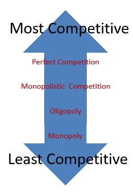
In the last review, we covered the perfectly competitive market structure. That is the most competitive of markets. Next, we will move on to the other extreme. Monopolies are the least competitive of markets. Review everything you need to know about monopolies on test day below.
Like All Profit Maximizing Firms:
- Produce the quantity where MR=MC
- Price at Demand
- Temporarily shut down when price falls below Average Variable Cost (AVC) at the profit maximizing quantity
- Profit/loss is determined by the gap between the ATC and the firm’s demand curve at the profit maximizing quantity (MR=MC)
Monopoly:
Number of Sellers: One. There are no close substitutes and no competitors.
Product Difference: The product is unique.
Barriers to Entry: High barriers which prevent any competitors from entering. Monopolies may engage in rent seeking behavior (working to pass voter initiatives, lobbying politicians, etc), to maintain a monopoly. These actions will increase the firm’s ATC and erode some economic profits.
Long-run Profit: Due to the high barriers to entry, economic profit is possible in the long run.
Ability to Impact Price: Monopoly power gives firms the ability to charge higher prices than would be charged in a competitive market. High barriers to entry are the driving force behind giving firms monopoly power.
Efficiency: No, Monopolies price above marginal cost and do not produce at the lowest average cost so they are not allocatively or productively efficient and they have deadweight loss.
Economies of Scale: Monopolies usually capture economies of scale because the profit maximizing quantity is on the downward sloping portion of their long-run average total cost curve.
Graph: Since there is only one firm, the market is the firm. As a result, the firms demand curve is downward sloping. The average revenue, and price will also be the demand curve (DARP). If the firm is a single price monopoly, the marginal revenue curve is below demand.
Note: The cost curves for a monopoly are the same as a perfectly competitive firm and monopolistically competitive firm. The AVC and AFC are rarely needed in this graph.

Why is the marginal revenue below demand?
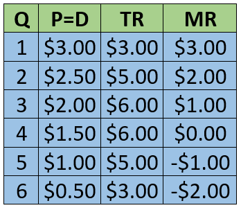
For a perfectly competitive firm (and a perfect price discriminating monopoly as seen below), marginal revenue is equal to demand. But for a single price monopoly (one that does not price discriminate), the marginal revenue is less than demand. That is because when the firm produces more output, it must lower the price of not just the last unit produced, but on all units produced. Take a look at the chart which shows the quantities of candy bars I could sell at each price (the demand is equal to the price). If I have one candy bar, I might be able to sell it for $3. But if I want to sell 2 candy bars, I must lower the price to $2.50; and since I am not a price discriminator, I charge the same price for both candy bars. As a result, the marginal revenue for that second candy bar isn’t the $2.50 I charged for it but just $2.00.
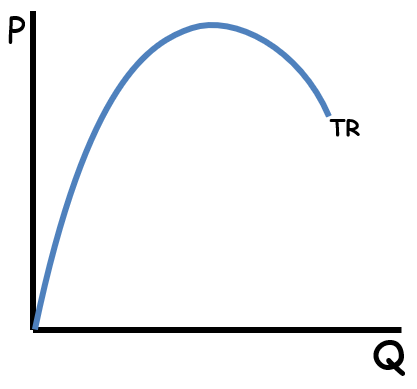
Total Revenue: As long as the marginal revenue curve is positive (above the x axis), total revenue is increasing as output increases. Since the marginal revenue curve is downward sloping, total revenue will increase at a decreasing rate. When marginal revenue is negative (below the x axis), total revenue decreases. So as output increases, a monopoly’s total revenue will increase at a decreasing rate, then decrease.
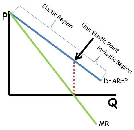
Marginal Revenue and Elasticity of Demand
The monopoly’s marginal revenue curve reveals the elasticity of the demand curve above. The total revenue test tells us a demand curve is elastic when a decrease in price causes an increase in total revenue. At lower quantities monopoly’s marginal revenue curve is positive. That means as price falls with each additional unit produced, total revenue increases. Therefore, the demand curve is elastic at those quantities. When marginal revenue is zero (where it intersects the x axis), the demand curve is unit elastic at that quantity because the decrease in price causes no change in total revenue. Finally, at higher quantities, the marginal revenue curve is negative which indicates total revenue decreases with the price decrease. As a result, that portion of the demand curve is inelastic. Profit maximizing monopolies will always produce in the elastic region of their demand curve.
Surplus and deadweight loss: Single price monopolies have both consumer and producer surplus. But since they do not produce the allocatively efficient quantity (where P=MC), they create deadweight loss and are inefficient.
Natural Monopolies and Regulation: A natural monopoly is an industry which captures economies of scale at the allocatively efficient quantity resulting in much lower average costs when there is a large single provider. These businesses usually have extremely high start-up costs but have a very low marginal cost of production. Electricity providers are a prime example of natural monopolies. The most expensive part of providing homes in a city with electricity is putting up wires and cables all over town to carry the electricity. If electric service was not a monopoly and consumers had multiple choices regarding who to purchase electricity from, the costs of production would be dramatically higher (as multiple sets of cables and wires would need to be strung) and price would likely be higher as a result. So, the natural monopoly may actually benefit consumers.
Governments will often regulate natural monopolies by imposing price ceilings which may be more efficient than the unregulated price. The socially optimal price is allocatively efficient and creates no deadweight loss where price equals marginal cost, but the firm may suffer economic losses at this price. If forced to earn economic losses, the firm will eventually exit the market so the government must provide the firm with a lump sum subsidy (equal to its loss) to eliminate deadweight loss.
A fair return price is one which enforces a price ceiling where economic profits are zero (P=ATC). At the fair return price, there is less deadweight loss than an unregulated monopoly and the firm breaks even.

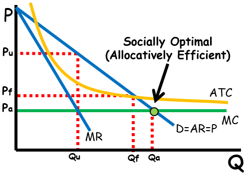
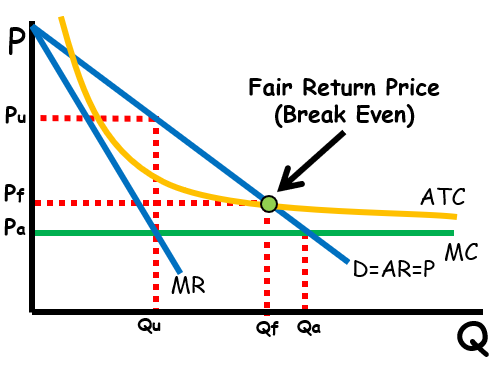
Compared to perfectly competitive markets: Unlike perfectly competitive firms, monopolies (as well as oligopolies and monopolistic competition) produce less, and price higher. Monopolies can also earn an economic profit in the long run.
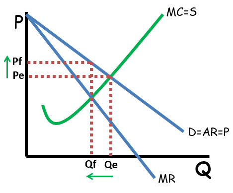
Price Discrimination: All of the monopolies above are called single price monopolies. That means they sell all units of output for the same price. Some monopolies are able to price discriminate and charge different prices for different units of output. Price discrimination occurs when a firm is able to charge different customers different prices for the same product. Letting kids eat free or giving senior citizens discounts at restaurants is an example of price discrimination.

Firms charge lower prices to people with a lower willingness to pay and higher prices to people with a higher willingness to pay. If the firm is able to figure out the maximum price each customer is willing to pay and charge them that price, the firm would be a perfect price discriminator. That would cause the MR curve to be the same curve as the Demand, Average Revenue, and Price (MRDARP). Perfect price discriminators are allocatively efficient. The last unit produced will be priced at the marginal cost.
Multiple Choice Connections:
2012 Released AP Microeconomics Exam Questions: 8, 9, 21, 24, 44, 53
Up Next:
Review Game: Product Market Structures Review, Shading Practice, and Prices, Points, and Quantities
Graph Drawing Practice: Monopoly and Monopolistic Competition
Content Review Page: Monopolistic Competition
Other recommended resources: ACDC Leadership (Monopoly)
