Everything you need to know about Oligopoly, Duopoly, and Game Theory
Updated 9/21/2021 Jacob Reed
Below you will find a breakdown of the oligopoly market structure. Make sure you practice the skills required to answer questions about this market structure with the Game Theory flash review when you finish reading.
Number of Sellers: A Few (ten or less). A Duopoly is an oligopoly with 2 firms.
Product Difference: Either. Products may be homogeneous or differentiated.
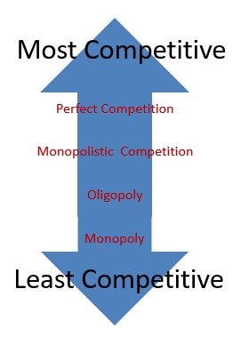
Ability to Affect Price: Yes. With oligopolies, there is usually a mutual interdependence between firms. The actions of one firm impact the actions (and profit) of other firms. Oligopolies are prone to collusion or the formation of cartels which set production quantities low and prices high. When cartels are successful oligopolies function as monopolies. Governments often regulate oligopolies and attempt to prevent collusion and cartels while encouraging competition through anti-trust laws. These anti-trust policies reduce monopoly power among firms. Fortunately, since there is an incentive to cheat, collusive agreements often break down even without anti-trust laws.
Barriers to Entry: High barriers which make it difficult for new firms to enter the market. Barriers include high start-up costs, government regulations, customer loyalty, etc.
Long-run Profit: Oligopolies often earn an economic profit in the long run due to high barriers to entry which prevent new firms from entering the market.
Efficiency: No, Oligopolies price above marginal cost and do not produce at the lowest average cost so they are not allocatively or productively efficient.
Graph: While there is a graph for oligopolies these firm’s behavior is better understood through game theory. As a result, a payoff matrix is used to determine outcomes.
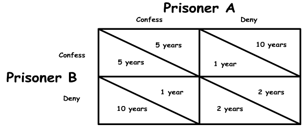
The Payoff Matrix: Game theory is the main way economists understands the behavior of firms within this market structure. Games consist of 2 players (in a duopoly which is all there is in Advanced Placement Microeconomics) each with two strategies. This creates a pay off matrix with 4 possible outcomes.
The trick to solving these problems is that you must put yourself in the mind of one actor while pondering how the actions of the second affect the decisions of the first. Mark the best decisions for each player as you go through the matrix. In the example below, green is used to mark the best decisions given the choice of the other player.
Take a look at the payoff matrix for the prisoners’ dilemma (see figure 1). In this classic game theory example two criminals are caught for stealing a car. The police also think they robbed a bank but they don’t have any evidence against them. The police separate the prisoners and question them individually. If they both confess to the bank robbery they both go to prison for 5 years. If they both deny robbing the bank, they both go to prison for 2 years. If one confesses while the other does not, the one who confesses will only go to prison for 1 year while the other will go to prison for 10 years. This scenario creates 4 possible outcomes illustrated in the 4 quadrants of the payoff matrix below.


Let’s look at prisoner A first. If prisoner A thinks prisoner B will confess, then prisoner A is deciding between confessing as well and getting 5 years in prison or denying and getting 10 years in prison (see figure 2). Confessing is a better option for Prisoner A.
If, on the other hand, prisoner A thinks prisoner B will deny, then prisoner A is deciding between confessing and getting 1 year in prison or denying and getting 2 years in prison (see figure 3). Again, confessing is the better option for prisoner A.

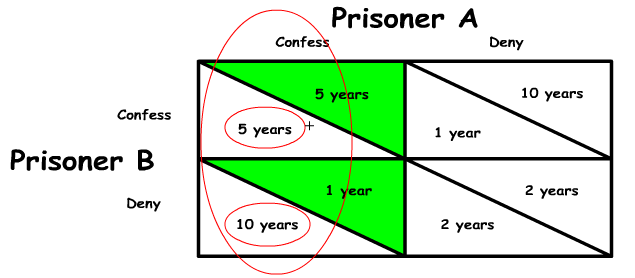
Now let’s look at prisoner B (see figure 4). If prisoner B thinks prisoner A will confess, then prisoner B is deciding between 5 years in prison (confessing also) or 10 years in prison (denying). Confessing is a better option for prisoner B.
If prisoner B thinks prisoner A will deny (see figure 5), then prisoner B is deciding between 1 year in prison (confessing) and two years in prison (denying). Again denying is the better option for prisoner B.
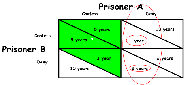
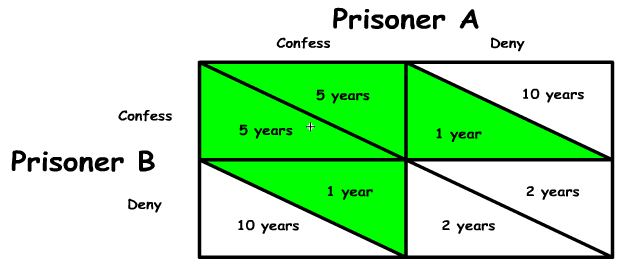
One thing you must know for these problems is the Nash Equilibrium. This is the most likely outcome if there is no collusion. It is also the quadrant containing two likely choices (upper left quadrant with 2 green triangles in figure 6 ). You should note, there is not always just one Nash Equilibrium; there could be two. Officially a Nash Equilibrium is defined as an outcome where neither firm has an incentive to change their behavior. In the prisoner’s dilemma above, the Nash Equilibrium is for both prisoners to confess. If either prisoner (not both) confesses, that prisoner would serve 10 years instead of 5. As a result, neither prisoner is likely to deviate from the Nash Equilibrium.
Occasionally you get a question asking about a Collusion outcome. This is much easier to figure out. For that you just look at all the quadrants in the pay off matrix and decide where the two entities would choose to end up if they could talk it out and come to some negotiated agreement. In our example that is the lower right quadrant where both prisoners deny and only spend two years in prison.
You also need to know what a Dominant Strategy is. This is the choice one of the players will make regardless of the other player’s action. In our prisoners’ dilemma, both prisoners have a dominant strategy to confess. That is both prisoners should confess regardless of what the other player does. You should note, there is not always a dominant strategy for a particular player. If there is not, it is because the actions of that player are dependent on the actions of the other player.
Multiple Choice Connections:
2012 Released AP Microeconomics Exam Questions: 11, 14, 39, 40
Up Next:
Review Game: Oligopoly Game Theory, Product Market Structures Review
Content Review Page: Diminishing Marginal Returns
Other recommended resource: Jason Welker
